General Algorithm in ANSYS APDL

Let’s define a general algorithm through which every design have to go through for its analysis. We will take a quick review of almost all the steps required for analysis in ANSYS APDL.

ANSYS APDL requires certain information about the model and analysis to be made. All requirements can be defined in three section.

1. Preprocessor
2. Solution
3. General Postprocessor

Preferences

Before explaining these sections, let’s see how preferences can help us in our work. There are many disciplines through which ANSYS analyses models. We normally work in one or two discipline at a time. When we check our relevant discipline in the preferences section, it tells ANSYS to narrow down options, questions and selections limited to those disciplines selected. This reduces our effort during further work on design analysis.

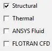
Preprocessor

As its name defines, in this section all the information about the model which are required for the solution are defined.

1. Element Type
2. Real Constants
3. Material Properties
4. Modeling
5. Meshing
6. Loads

Element Type

Here we can add elements which we will be using for our model. Degrees of freedom can be restricted right from here or may be left as we can narrow it down later as well.

There can be many type of elements. Once an element is defined here, later relevant dimension should be required for analysis i.e. width and height for beam; internal and external diameters for pipe etc.

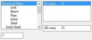
Real Constants

Here we can make ‘real constant sets’, which means a set of real constants that can be applied on any compatible element. Before we start, we have to select one of the predefined element so that ANSYS can ask relevant information about that kind of element.

A Reference No is allotted to this set of real constant so that later we can use it to assign these set of properties on any of the available elements in our model for analysis.

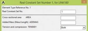
Material Properties

As the section name says, we will enter material properties that ANSYS requires for its analysis. As we define these properties for a material, a ‘Material Number’ is assigned to these properties which we can later assign to any element we want.

Sections

Here we define section of our element. It mainly includes cross sectional dimensions of elements.

For instance, for a beam, breadth and height have to be defined. For every dimension set, an ‘ID’ is assigned so that we can later assign it to any element we want in our model.

Modeling

In this section we model our required geometry for analysis. We make geometry according to our problem statement.

Here one important point should be made clear. ANSYS analyses all models on [NODE/ELEMENT] basis. If we model key points, lines, areas etc. ANSYS does not know how to distribute the applied loads on these sections. So it divides it into nodes and elements (Meshing) then applies analysis calculations on it.

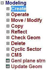
We have two options here. We can either draw key points then join them to make lines, areas etc. which will be converted to nodes and elements in meshing section or we can directly draw nodes and assign elements to them.

Meshing

As discussed earlier, here ANSYS converts all modelled parts into nodes and elements. For this it requires us to define which key points, lines, areas should be meshed for analysis. And how many nodes we want to make. As number of nodes increases, the precision of our result increases.

Loads

After meshing, one last thing which is left is to apply loads. Loads can be displacements, forces, moments, temperature and even Q_in, Q_out etc in other type of analysis. These loads can be of constant magnitude or can be of variable in nature. It can be defined as a function of some other variables as well.

Before we apply any load, we have to decide which type of analysis we want from it. We define analysis first. There are several kind to analysis ANSYS can do but ‘Static’ and ‘Transient’ are commonly required.

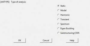
After setting analysis, we define loads. Its type depends on our need. These loads are applied to certain key points, nodes or on other places where they are applicable. Structural displacements means restrictions we want like wall joint in a cantilever beam etc.

Now the preprocessor is completed. All required data is provided to ANSYS for its analysis.

Solution

Analysis type and loads can be defined here as well. But usually this section is used for solving the analysis problem.

1. Analysis Type
2. Define Loads
3. Solve

Here we will discuss only solve section as analysis and loads are already discussed earlier.

Solve

We usually solve ‘Current Load Step’ (LS). Before we solve, ANSYS wants us to have a look on solution options and load step options. When we press ‘OK’ it starts evaluating the solution. That’s it!

General Postprocessor

Here we can extract the result of our analysis in many aspects, raw and summarized.

Plot Results

We can plot results in a variety of graphical ways.

Deformed shape can be seen in three ways

1. Deformed shape
2. Deformed and unreformed shape
3. Deformed and unreformed edge

Contour Plot have several options like nodal solution or element solution. As analysis is based in nodes and elements, results can be evaluated in either form.

There are a lot of analytical solutions which can be evaluated from ANSYS. It depends upon our need that what it requires for further design, comparison or analysis.

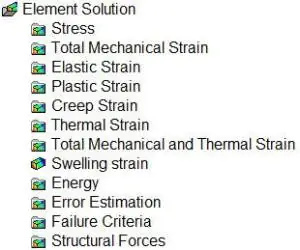
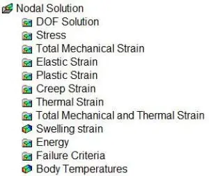
Contour plots are displayed in sections with similar properties. There is a scale which relates colors with magnitude of change or other property.

That’s how a general problem in solved. From now on we will solve typical problems and discuss its solution in ANSYS – Mechanical APDL.