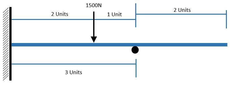
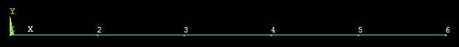
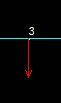
Let’s solve a structural beam analysis problem. Suppose there is a cantilever beam. It is attached to wall at one end while other end is free. Problem Diagram is shown above. Other details are also written along the diagram. A force is applied on it with a magnitude of 1500N downwards. A support is provided 3 units away from the wall. Diagram has clearly defined the position of all constraints.
Below is quick to-do list which we will go through to solve our problem in Mechanical APDL.
- Preferences
- Preprocessor
- Define
- Element
- Material Properties
- Section
- Create nodes
- Define Element through nodes
- Define Analysis
- Apply Loads
- Define
- Solution
- Solve LS
- General Postproc
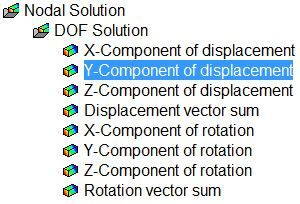
- Nodal Solution
Let’s start out analysis.
We will set this to ‘Structural’. This is because all our constraints are 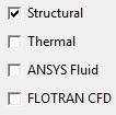 structural. And we don’t want other disciplines option to show up as they will mess things up.
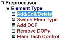
Our element is beam 188 so we will add an element in preprocessor.
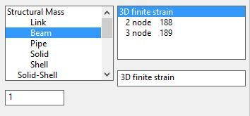
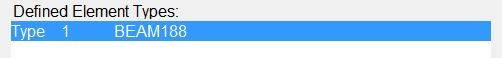
Notice the Number 1 written between ‘Type’ and ‘BEAM188’. This is the reference number which assigned to this element. It can be later to refer this element.
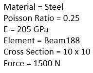
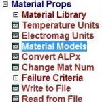
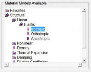
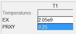
Now we will enter material properties. We have Young’s Modulus of magnitude 2.05e9 and Poisson Ratio 0.25.
Before we enter these valued we have to define certain classes which are necessarily required by ANSYS for its calculations. In our case, it is a structural linear elastic isotropic problem. ANSYS assumes these properties to be ideal and does its calculations taking our values of material properties.
These material properties along with their magnitude are also assigned with a number. So that we can later relate elements with their properties as there can be many elements having different properties.
Now we will define section. It is the cross section of our beam which is required to be defined here. Notice the ID number assigned to this section. This ID would be later used to define element cross section.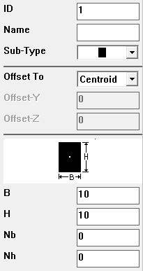
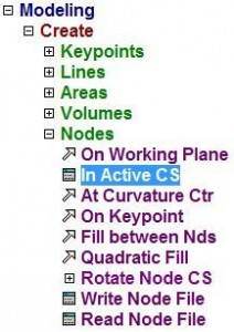
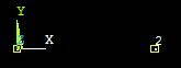
First part of modeling is to create nodes. In our case, there are six nodes. We will active coordinate system. Fill in all the nodes as first three are filled in the pictures below.
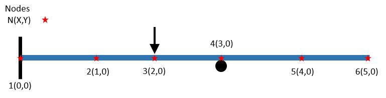
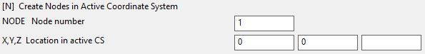
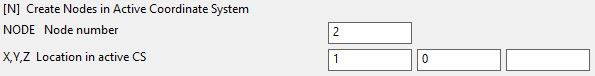
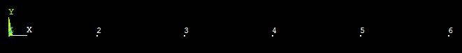
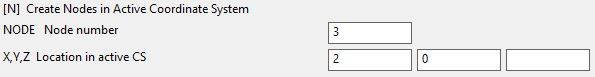 Notice the linear pattern of the nodes as our beam is straight. For curved surfaces, nodes will be entered accordingly.
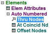
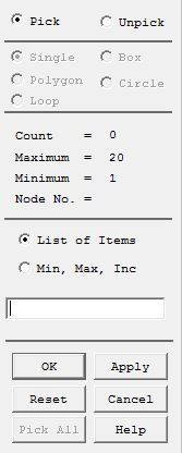
After defining loads, we will define element through nodes. If tells APDL that there is X-element between so and so node. In our case X is equal to 1. To define elements, two nodes at a time is selected if list of items is checked.
First click ‘Thru Nodes’. Then click on node 1 which is at the XYZ center. Now click the node 2. Now click apply. Notice the line between the nodes. It shows that something is now defined between these two nodes. Now do this for node 2 and 3. Then for 3 and 4 and so on.
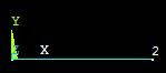
There should be a straight line at the end of this part.
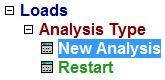
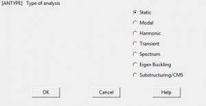
Now we will apply loads on these nodes. Firstly we have to create an analysis which APDL will perform as our is defined now. In our case, the analysis is ‘Static’ as all our loads are static.
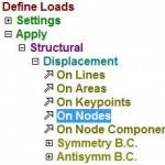
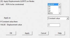
Now at node 1, as this end is attached to wall, a displacement constraint of ALL DOF (Degree of Freedom) should be introduced with a magnitude of ‘0’. As this end of beam cannot move in any direction. First click ‘On Nodes’ then select the node where load/constraint is to be applied, then click apply. In new dialog box, select ALL DOF and enter ‘0’. Notice the arrows at node 1 after placing the constraint. It shows how the beam is restricted at this end.


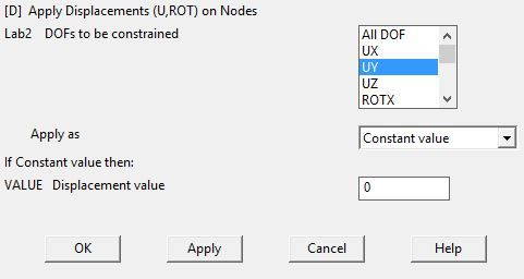
Now we will apply the constraint at node 4. As at this point, a vertical support restrains vertical motion i.e. in y axis. Notice the the horizontal arrow which shows that the beam is horizontally restricted at this point.

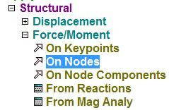
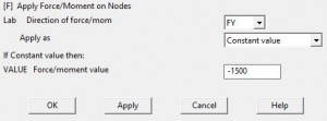
One last load is left which is a force load of magnitude 1500 in negative y direction. Notice the arrow after applying the load. Its direction is according to the direction of force.
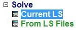
As all constraints are applied, now we will solve this. A dialog box appears as we click ‘Current LS’. This gives details of our problem as we have defined it APDL and ask us to confirm it.
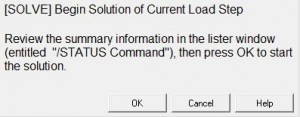
As we press ‘OK’ it will start the solution. ‘Solution is done!’ dialog assures that solution is done accordingly and no errors were found. If APDL finds any error or anomaly, it states here. Sometimes we can ignore it but sometimes error are unacceptable and we have change our inputs accordingly to remove that error.

To view the results of our problem, we go to General Postproc. There can be any solutions possible. It is our need that defines which we require to do further calculations.

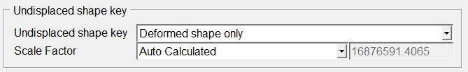
This undisplaced shape key can be used to view both undeformed and deformed shape of beam simultaneously for comparison.
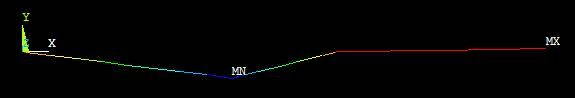
Along with the results in contour form, there is a scale which used to read results. ANSYS use different colors to define and show different sections of element with varying property. Part of beam with same color shows that it has the same magnitude of that property. Notice the abrupt change in beam even after we have defined it as elastic. This is so because it has a very poor nodal resolution. If many hundreds of nodes were defined between these nodes, the result could be very changed. But here, the objective is to demonstrate the use of APDL for analyzing such situations.
 That’s all!. Below is a video which shows all the steps described above. Hope you find the article and video helpful.
Share it
Leave a Reply